Withdrawal Rates, CAGR and Volatility

We discussed the dangers of planning one’s retirement journey using average compounding rates in a previous post. In this post, I will try to quantify what we discussed earlier.

I’ll start with a variety of withdrawal rates. Let me once again define the withdrawal rate for clarity. The withdrawal rate is the portion of the overall corpus one withdraws in the first year of retirement. Once that amount is determined, we keep withdrawing the same amount adjusted for inflation every year for the duration of the planned period. For example, if the corpus is Rs. 1 crore and the first-year withdrawal is Rs. 4 lakh, then the withdrawal rate is 4%. The next year, we will adjust the Rs. 4 lakh based on inflation and withdraw it irrespective of what the corpus is. We would keep doing the same year after year until the corpus depletes to zero at the end of the planned period.

In Fig. 1, I’ve listed different withdrawal rates in the columns and retirement periods in the rows. The assumed inflation rate is 7%. Remember, these are just the average returns and a starting point for retirement planning. The reason these are listed here is to provide a sense of the relationship between withdrawal rates and retirement years. Each cell represents the constant returns needed to meet the target retirement years for a withdrawal rate.

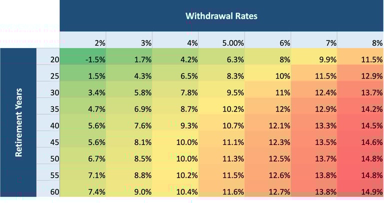
Fig.1 Constant returns on corpus for different withdrawal rates and retirement timelines

As one can see, the lower the withdrawal rate and retirement years (left top), the lower the returns needed on the corpus to cover the withdrawals. With the current risk-free rates of 7% (10-year government treasury), we can easily navigate 55 years with a 2% withdrawal. However, as we move to the right, 7% covers a shorter period than before. Just moving from 2% to 3% reduces the retirement period to 35 years. For any withdrawal rate beyond 5%, a 7% return does not even cover 20 years of retirement.

The NSE 500 (the broadest index for the Indian market covering a range of large, mid, and small-cap companies, representing around 96% of our market capitalization) gave around 13% average returns between 1995 and 2024. If it had given exactly 13% year on year every year like a FD or Bond(which is not true in real life), one can sustain even a 7% withdrawal rate for 35 years. For any withdrawal rate of 6% or below, the retirement fund would never run out (as long as inflation remains 7% or lower). We discussed this earlier.

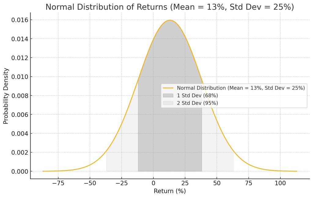
Now, don’t let the lure of 13% CAGR trick you into investing all your corpus into the NSE 500 index. Doing so could be detrimental to one’s financial retirement, as we will now discuss. That’s because even though the average returns may be 13%, they vary from one year to the next due to Volatility.

Standard deviation (sdev) is the measure of volatility. During the last three decades, the annualized volatility for the NSE 500 Index is a nerve-wracking 25%. This means around two out of three years, the market returns are between 13% + 25% = 38% up and 13% - 25% = -12% down. One of those three years, it may go up or down beyond the -12% to +38% range.

What do these numbers mean to our retirement journey? For that, refer to Fig. 2. Let me first discuss how to read these statistics and the approach to calculating them. We already know that the average returns for the NSE 500 are 13%. Now, assume one invests all their corpus in the NSE 500. Once invested, we pick a withdrawal rate as above from 2% to 8% and a retirement period ranging from 20 to 50 years. What we see in individual cells is the sdev that gives us a 90% success rate of making it through the retirement years with the average 13% CAGR.

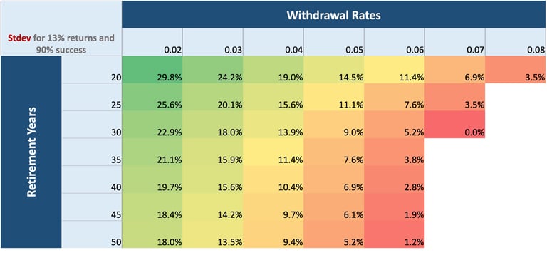
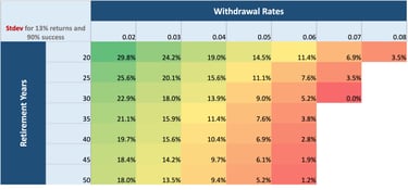
Fig.2 With 13% average returns, the acceptable volatility(stdev) for 90% of the withdrawal rates

Let’s take an example. Assume a withdrawal rate of 4% and a retirement period of 30 years. Reading from the table, we get an sdev of 13.9%. This represents the sdev for securing a 90% chance that we can make it through 30 years of retirement without running out of money. For us to succeed, the market can’t keep swinging from -12% to 38% anymore. It needs to move between a narrower range of (13% + 13.9% = 26.9% up) and (13% - 13.9% = -0.9% down). The higher the withdrawal rate or retirement period, the tighter the market range must be to ensure 90% success. For a 30-year period and a 7% withdrawal, we need the market to behave almost like a fixed deposit giving a 13% rate. For a 7% withdrawal, a 13% return can’t sustain beyond 30 years with the same 90% success. To stretch beyond, we need to accept a lower success rate.

A similar table can be built keeping sdev constant to determine the CAGR needed for success. The message is clear: retirees need high returns and low volatility for a successful retirement journey. But the real world is just the opposite. Typically, high returns come packaged with high volatility, and low guaranteed returns do not go very far. One needs to carefully pick asset classes and products to construct a robust portfolio. Essentially, retirement planning is about mixing various asset classes such as bonds, equity, gold, cash, crypto, etc., to increase returns while reducing volatility. Diversification is important even during the working years. For retirement planning, diversification is absolutely critical.

There are tools available that can help with diversification by building scenarios for what-if analysis and running them through simulations. Simulation plays a big part in building the right portfolio mix. The above analysis was done using Monte Carlo simulation. With the help of data points like CAGR and sdev, one can create hundreds or even thousands of Monte Carlo iterations. These iterations help with assessing the rate of success for any portfolio under different conditions such as different withdrawal rates, retirement periods, and inflation rates. One can also build in conditions like emergency withdrawals, moratoriums on withdrawals, conditional withdrawals, etc. I’ll cover these in future posts.